In this project, I implemented a physically-based renderer using a pathtracing algorithm. In other words, I implemented code to model the path of light in a scene. To do so, I first wrote code to generate a ray from the perspective of a camera, and used that ray to determine its intersections with primitive objects in a scene, such as triangles and spheres. To speed up this process, I used a bounding volume hierarchy to find an intersection faster, so I wouldn't have to traverse every primitive in a scene to find one. Then, I implemented direct illumination by modeling the path of light that falls directly from a light source onto an object. Next, I implemented global illumination by integrating direct and indirect lighting. Finally, I used adaptive sampling to improve efficiency and reduce noise in my renderings.
Part 1: Ray Generation and Scene Intersection
To generate a ray, I took in two doubles, x and y, that represent a point in image space from (0,0) to (1,1), and converted the 2D point into a 3D point in camera space. I did this by multiplying the x and y coordinates by the width and height of the camera space, and adding the values to the x and y values of the bottom left corner of the camera space. For the z value of the 3D vector, I used -1. I generated a ray in camera space using the new vector as its direction, and the position of the camera as its origin. I converted the ray into world space by multiplying it by the camera to world transformation matrix.
Once I generated a ray, I used the ray to find if it intersected a triangle by using the Möller-Trumbore algorithm. The Möller-Trumbore algorithm is used to solve a system of equations to find three unknowns, t, u, and v. It works by writing the intersection point in both barycentric coordinates and in terms of the ray. The three weights of the barycentric coordinates are represented as u, v, and 1 - u - v, while the ray equation is written as ray origin + ray distance * t. The two equations can be set equal each other, and Cramer's rule can be applied to solve the system of equations. After using the Möller-Trumbore algorithm, which is derived using Cramer's rule, I checked for triangle intersection by chacking to see if the 't' value was positive and between the given ray's minimumum and maximum time values. If it was, I set the intersection object's time value to t. I set the intersection object's primitive value using the this object, the bsdf by using get_bsdf(), and the normal by multipling the normals of the triangle by the barycentric coordinates derived using Möller-Trumbore.
|
|
|
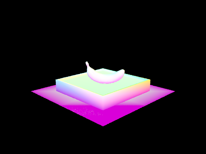
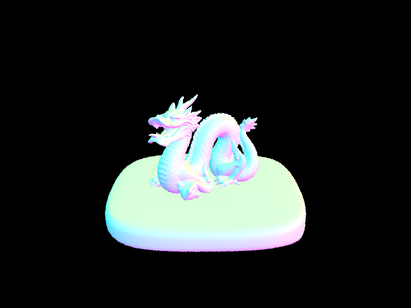
Normal shading for some small .dae files.
Part 2: Bounding Volume Hierarchy
For the bounding volume hierarchy, I used a recursive code to traverse a series of bounding boxes to find the intersection with a ray and a primitive. To construct a bounding box, I took all the centroids of the primmitives and put them in a new bounding box by using the expand method. I then found the split point by iterating through each axis and finding the longest one by using the extent method. I set the split point to be the centroid of the longest axis. If the amount of primitives is smaller than the maximum size for leaf nodes, I set the bounding box node to be a leaf by setting its start and end pointers to the given start and end primitives, and simply returning the node. If the node was not a leaf node, I split the primitives into a left vector iterator and a right vector iterator depending on which side of the split point their centroids were on. I then called the bvh constructor recursively to create the left child node, where I set the start and end iterators to be the start and end of the left vector primitives, and did the same for the right child node with the right vector primitives.
When intersecting scenes without BVH, such as the banana dae, I averaged 2458.000000 intersetion tests per ray at an average speed of 0.0152 million rays per second, while with BVH, I averaged 0.989437 intersection tests per ray and 0.4198 million rays per second. For the teapot dae, without the bvh I averaged 2464.000000 intersetion tests per ray at an average speed of 0.0082 million rays per second, while with BVH, I averaged 2.615852 intersection tests per ray and 0.2793 million rays per second. Thus, the BVH improved the speed of rendering tremendously. Without BVH, we have to traverse every primitive in a scene in order to find an intersection, while with BVH, we can narrow down the number of primitives to iterate through by checking intersections with larger bounding boxes first.
|
|
|
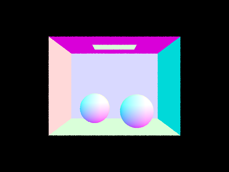
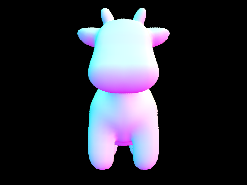
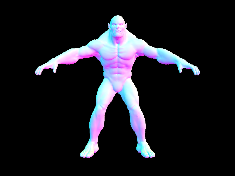
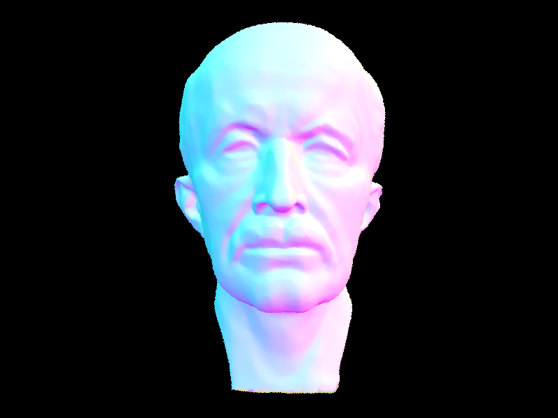
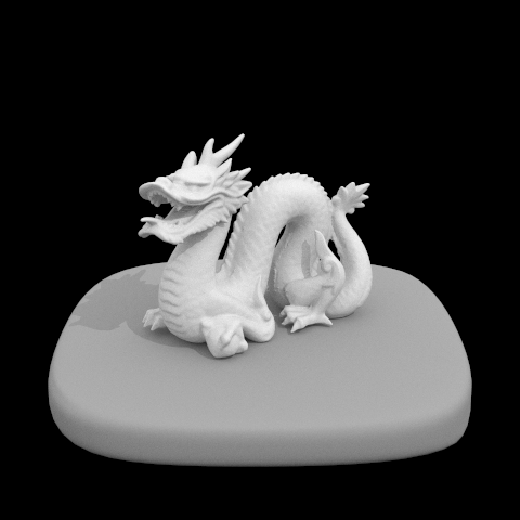
Shading for some large .dae files that could only be rendered in reasonable time with BVH acceleration.
Part 3: Direct Illumination
I implemented two direct illumination functions, estimate direct lighting with uniform hemisphere sampling, and estimate direct lighting by importance smapling lights. Direct lighting only calculates light that falls directly from a light source onto an object. For uniform hemisphere sampling, I iterated through the number of lights in the scene multiplied by ns_area_light. For each light, I got a sample for an incoming ray by calling hemisphereSampler -> get_sample(), converted this ray by multiplying it by the object to world matrix, and created a new ray using the newly calculated ray as its distance and the hit point as its origin. I then checked if the new ray intersected with the bounding volume hierarchy, and filled an intersection object if it did. If there was an intersection, I added the reflectance equation with the relevant inputs for the ray to a running sum I called L_out. At the end, I returned L_out divided by the number of samples and the pdf, which remained constant for uniform hemisphere sampling.
For estimating direct lighting with importance sampling, I still iterated through all of the lights. I first checked to see if the light was a delta light, and assigned its number of samples to be 1 if so and to be ns_area_light if otherwise. Then, I iterated through the number of samples per light, and generated a ray like in hemisphere sampling. However, I checked to see if the ray intersected with any objects in the scene to determine if it had a direct path to the light, and updated L_out if the ray did not intersect with the bvh. For each light, I divided L_out by its number of samples, and returned L_out at the end.
|
|
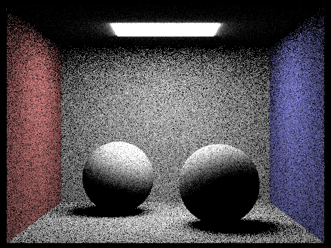
 Results of images sampled with hemisphere sampling.
|
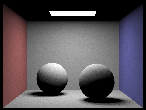
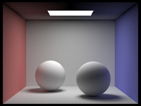
 Results of images sampled with importance sampling.
|
 Rendering with 1 light ray.
|
 Rendering with 4 light rays.
|
 Rendering with 16 light rays.
|
 Rendering with 64 light rays.
|
Uniform hemisphere sampling yields more noise than importance sampling does. This is likely due to the fact that importance sampling only samples from the lights in the scene.
Part 4: Global Illumination
Indirect lighting includes light that bounces off of objects, not the light directly from a light source like in direct lighting. To implement indirect lighting, I used the function at_leat_one_bounce_radiance, which initially set L_out to be the one_bounce_radiance value, generated an incoming vector and a pdf by calling sample_f from the intersection object's bsdf, and used the concept of Russian Roulette to terminate recursion. If Russian Roulette variable, a random variable that returns true with a probability of 65%, returns true, and if the ray is not at its maximum depth, the functioni at_leat_one_bounce_radiance is called recursively. Otherwise, it is terminated and L_out is returned.
|
|
|
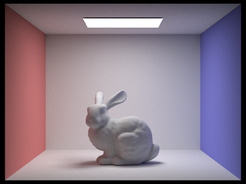
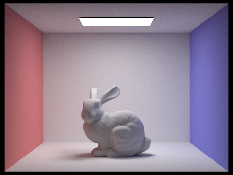
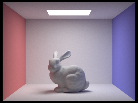
Images rendered with global illumination with 1024 samples per pixel.
 Bunny rendered with only direct illumination.
|
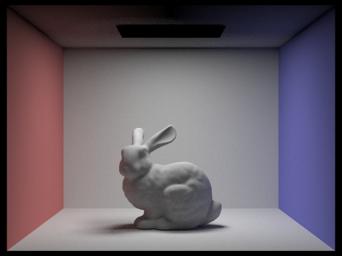 Bunny rendered with only indirect illumination.
|
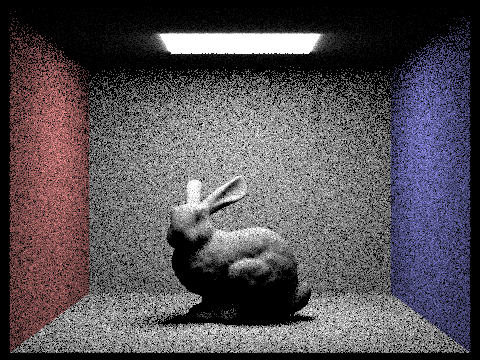
 Bunny rendered with max_ray_depth of 0.
|
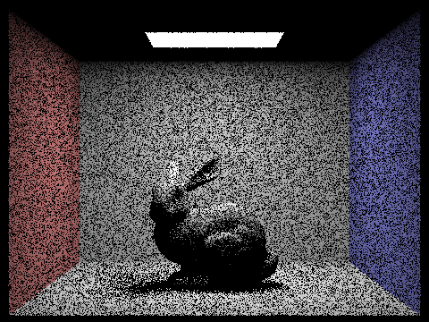
 Bunny rendered with max_ray_depth of 1.
|
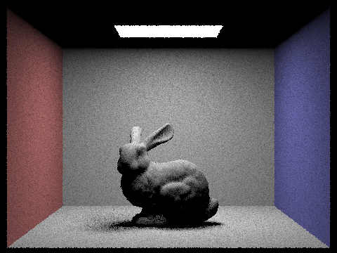
 Bunny rendered with max_ray_depth of 2.
|
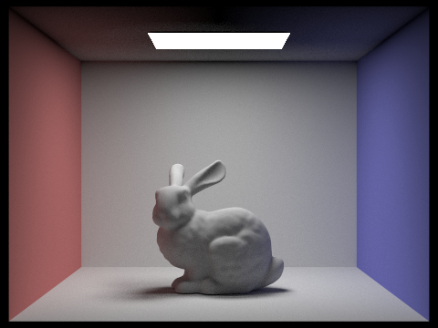
 Bunny rendered with max_ray_depth of 3.
|
Shading for some large .dae files
 Bunny rendered with max_ray_depth of 100.
|
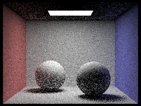 Spheres rendered with sample-per-pixel rate of 1.
|
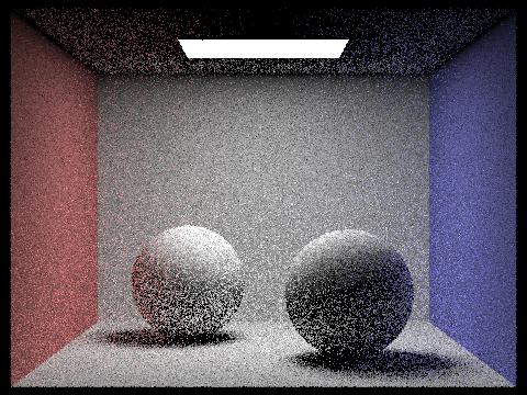 Spheres rendered with sample-per-pixel rate of 2.
|
 Spheres rendered with sample-per-pixel rate of 4.
|
 Spheres rendered with sample-per-pixel rate of 8.
|
 Spheres rendered with sample-per-pixel rate of 16.
|
 Spheres rendered with sample-per-pixel rate of 64.
|
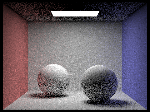
 Spheres rendered with sample-per-pixel rate of 1024.
|
Part 5: Adaptive Sampling
I implemented adaptive sampling by altering my raytracing function. I checked every 32 samples to see if the samples had converged. I did this by calculating the mean and the variance of the samples so far, by using values s1 and s2 which are running sums of the illum() function and of the square of the illum() function, which is generated from the spectrum created by calling est_radiance_global_illumination on the generated ray. Using variance, I calculated the variable I, which is 1.96 * the square root of the variance divided by the number of samples so far. To check for convergence, we want this value I to be less than the maxTolerance multiplied by the mean. If I is less than or equal to this value, we break out of the sampling loop because the value has converged.
 Bunny rendered with 2048 samples per pixel.
|
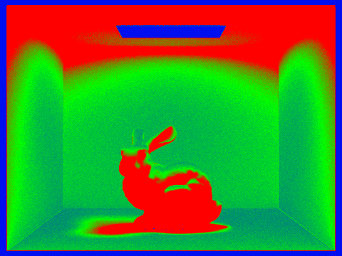 Sample rate of bunny.
|